Building a Smith Chart in JavaScript: Inside the Rendering Pipeline
See how SciChart.js was extended to build a fully interactive Smith chart using standard APIs. This article highlights the flexibility of custom rendering and advanced interactions.
It’s been a topic I’ve wanted to write about for a while, how SciChart – High Performance Realtime Charts is actually much more than a chart component, it can be used for advanced graphics & visualisation in many different sectors, but I lacked the good example to demonstrate the flexibility and power of SciChart.
In this blog post I’m going to walk you through the following:
Read on to find out how we did this!
So here was the idea I had. What about visualising 3D LiDAR data in SciChart? LiDAR data can be collected from a variety of sources: UAV drones (Unmanned Aerial Vehicles), self-driving cars, geological survey tools and more.
It can be used in a variety of scenarios: anything from defence/tactical operations to geological survey such as energy/mining, geospatial analysis, civil engineering, construction and more.
The power to visualize LiDAR / Geospatial data is sitting in most of our pockets in the form of an iPhone or Android phone, or in our cars or offices in the form of a tablet or laptop. Modern phones really are powerhouses of computing, often with quad-core processors and dedicated GPUs. You will be surprised with what you can do with one of these devices when paired with powerful graphics and visualisation software such as SciChart.
The problem I had was where to get a dataset. What is the dataset format? How large are the dataset files?
Well, I basically googled ‘LiDAR Dataset’ and the first link was a UK Government site with LiDAR composite data for the entire United Kingdom. OK, That’s probably a big dataset … Luckily they had a nice website where you could select a region and download sub datasets.
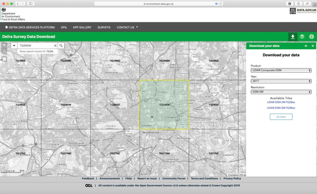
I thought what would be an interesting location and decided on Central London. Zooming in to tile TQ38SW I grabbed a dataset of a 20 1km x 1km square tiles containing ASC (Ascii GIS format) files.
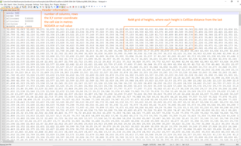
The ASC file format is pretty simple. It’s just a text-file which contains some header parameters then a uniform grid of heights. Each height is a floating point number corresponding to the altitude in metres. Each height-value is spaced CellSize metres from the previous, so you can consider the ASC file as a uniform NxM matrix or grid of heights. This is perfect, it corresponds perfectly to SciChart data formats :)
So the C# code to read an ASC LiDAR file took me about half an hour to write, as it’s not a particularly complicated file format and entirely text based. The code is included below.
using System;
using System.Collections.Generic;
using System.Globalization;
using System.IO;
using System.Linq;
using System.Threading.Tasks;
using System.Windows.Media;

namespace SciChart.Lidar3DPointCloudDemo
{
    public struct AscData
    {
        public List<float> XValues { get; set; }
        public List<float> YValues { get; set; }
        public List<float> ZValues { get; set; }
        public List<Color> ColorValues { get; set; }
        public int CellSize { get; set; }
        public int XllCorner { get; set; }
        public int YllCorner { get; set; }
        public int NumberColumns { get; set; }
        public int NumberRows { get; set; }
        public int NoDataValue { get; set; }
    }

    public class AscReader
    {
        public static async Task<AscData> ReadFileToAscData(
            string filename, Func<float, Color> colorMapFunction, Action<int> reportProgress = null)
        {
            AscData result = new AscData()
            {
                XValues = new List<float>(),
                YValues = new List<float>(),
                ZValues = new List<float>(),
                ColorValues = new List<Color>(),
            };

            await Task.Run(() =>
            {
                using (var file = File.OpenText(filename))
                {
                    // Load the ASC file format
                    result.NumberColumns = ReadInt(file, "ncols");
                    result.NumberRows = ReadInt(file, "nrows");
                    result.XllCorner = ReadInt(file, "xllcorner");
                    result.YllCorner = ReadInt(file, "yllcorner");
                    result.CellSize = ReadInt(file, "cellsize");
                    result.NoDataValue = ReadInt(file, "NODATA_value");

                    // Generate X-values based off cell position
                    float[] xValuesRow = Enumerable.Range(0, result.NumberColumns).Select(x => (float)x * result.CellSize).ToArray();

                    for (int i = 0; i < result.NumberRows; i++)
                    {
                        // Read heights from the ASC file and generate Z-cell values
                        float[] heightValuesRow = ReadFloats(file, " ", result.NoDataValue);
                        float[] zValuesRow = Enumerable.Repeat(0 + i * result.CellSize, result.NumberRows).Select(x => (float)x).ToArray();

                        result.XValues.AddRange(xValuesRow);
                        result.YValues.AddRange(heightValuesRow);
                        result.ZValues.AddRange(zValuesRow);

                        if (colorMapFunction != null)
                        {
                            // Optional color-mapping of points based on height
                            Color[] colorValuesRow = heightValuesRow
                                .Select(colorMapFunction)
                                .ToArray();
                            result.ColorValues.AddRange(colorValuesRow);
                        }

                        // Optional report loading progress 0-100%
                        reportProgress?.Invoke((int)(100.0f * i / result.NumberRows));
                    }
                }
            });

            return result;
        }

        private static int ReadInt(StreamReader file, string prefix)
        {
            string line = file.ReadLine();
            line = line.Replace(prefix, "").Trim();
            return Int32.Parse(line, CultureInfo.InvariantCulture);
        }

        private static float[] ReadFloats(StreamReader file, string separator, float noDataValue)
        {
            string line = file.ReadLine();
            float[] values = line.Split(new[] {separator}, StringSplitOptions.RemoveEmptyEntries)
                .Select(x =>
                {
                    float rawValue = float.Parse(x);
                    return rawValue == noDataValue ? float.NaN : rawValue;
                } ).ToArray();
            return values;
        }
    }
}
In this class ASCReader we have an async method ReadFileToAscData:
public static async Task<AscData> ReadFileToAscData(
            string filename,
            Func<float, Color> colorMapFunction,
            Action<int> reportProgress = null)
This function accepts a filename, an optional callback function to map a height to a colour, and an optional callback to report progress from 0…100% on the loading operation. It turns out loading a single ASC LiDAR file from the Defra Survey takes a very short time but the whole method is async and setup for much larger files if you have them.
Once the data is loaded, in this case into a struct called AscData, which looks as follows:
public struct AscData
{
public List<float> XValues { get; set; }
public List<float> YValues { get; set; }
public List<float> ZValues { get; set; }
public List<Color> ColorValues { get; set; }
public int CellSize { get; set; }
public int XllCorner { get; set; }
public int YllCorner { get; set; }
public int NumberColumns { get; set; }
public int NumberRows { get; set; }
public int NoDataValue { get; set; }
}
This struct contains all the data we need, including a List of X,Y,Z values (as floats), ColorValues (this list will be empty if you don’t pass a colormap function to the AscReader) as well as other header information such as CellSize which specifies the spacing in metres between each data-point, XllCorner, YllCorner which specify the location of the top-left cell in the ‘world’, Number of columns/rows and the NoDataValue or null value.
For SciChart visualizing we transformed the NoDataValue to float.NaN, as SciChart is already setup to render NaN as a gap. We used floating-point datatype not double because the extra-precision of 64-bit is not needed for this example, and float uses half the memory, so why not.
Finally, we had to transform the ASC dataset to SciChart data types, and this part proved quite easy due to our flexible API for drawing 3D point-clouds and contour/topology maps.
// Transforming AscData to SciChart XyzDataSeries3D for point-clouds
//
public static async Task<XyzDataSeries3D<float>> ParseToXyzDataSeries(AscData lidarData)
{
var xyzDataSeries3D = new XyzDataSeries3D<float>();

await Task.Run(() =>
{
if (lidarData.ColorValues.IsNullOrEmpty())
{
            // When no Color map, just append XYZ points
xyzDataSeries3D.Append(lidarData.XValues, lidarData.YValues, lidarData.ZValues);
}
else
{
            // When a Color map exists, append XYZ points and colour data
xyzDataSeries3D.Append(lidarData.XValues, lidarData.YValues, lidarData.ZValues, lidarData.ColorValues.Select(x => new PointMetadata3D(x)));
}
});

return xyzDataSeries3D;
}
We opted to choose a colour map and our ColorMapFunction simply mapped from height to a gradient brush, which we’ll talk about below. This gives the added benefit of immediately being able to see the approximate elevation of items of interest based on the colour, which adds a fourth dimension to the visualisation.
The XyzDataSeries3D datatype in SciChart can be visualized with a point-cloud chart using the following code.
XAML
In the XAML we declare a SciChart3DSurface, add an X,Y,Z axis and set some ChartModifiers for zooming, panning and orbiting the view.
<s3D:SciChart3DSurface x:Name="SciChart3DSurface" WorldDimensions="1000,200,1000">

<s3D:SciChart3DSurface.Camera>
<s3D:Camera3D FarClip="10000" Position="800,1000,800"/>
</s3D:SciChart3DSurface.Camera>

<s3D:SciChart3DSurface.RenderableSeries>

<!-- Renders the point cloud -->
<s3D:ScatterRenderableSeries3D x:Name="pointCloud">
<s3D:ScatterRenderableSeries3D.PointMarker>
<s3D:PixelPointMarker3D Fill="LimeGreen"/>
</s3D:ScatterRenderableSeries3D.PointMarker>
</s3D:ScatterRenderableSeries3D>
</s3D:SciChart3DSurface.RenderableSeries>

<s3D:SciChart3DSurface.XAxis>
<s3D:NumericAxis3D TextFormatting="0m" AxisTitle="X Distance (metres)" />
</s3D:SciChart3DSurface.XAxis>
<s3D:SciChart3DSurface.YAxis>
<s3D:NumericAxis3D VisibleRange="0, 50" TextFormatting="0m" AxisTitle="Height (metres)" />
</s3D:SciChart3DSurface.YAxis>
<s3D:SciChart3DSurface.ZAxis>
<s3D:NumericAxis3D TextFormatting="0m" AxisTitle="Y Distance (metres)" />
</s3D:SciChart3DSurface.ZAxis>

<!-- Enables interaction such as orbit, or movement on W-A-X-D key down -->
<!-- Double click to reset zoom -->
<s3D:SciChart3DSurface.ChartModifier>
<s3D:ModifierGroup3D>
<s3D:OrbitModifier3D/>
<s3D:FreeLookModifier3D ExecuteWhen="Ctrl" MovementSpeed="20"/>
<s3D:MouseWheelZoomModifier3D/>
<s3D:ZoomExtentsModifier3D ResetPosition="800,1000,800" ResetTarget="0,25,0" AnimateDurationMs="500"/>
</s3D:ModifierGroup3D>
</s3D:SciChart3DSurface.ChartModifier>

</s3D:SciChart3DSurface>
Code-behind
In the code-behind we load the ASC File using the AscReader class and setup our colour-map using SciChart’s LinearColorMap class to convert each height-value into a linearly-interpolated colour in a gradient that we provided. The Gradient is mapped from 0 to 50 so in this example elevation 0m or below maps to DodgerBlue, while elevation 50m or above maps to Purple.
public partial class MainWindow : Window
{
public MainWindow()
{
InitializeComponent();

ReadLidarData();
}

private async void ReadLidarData()
{
// The LinearColorMap type in SciChart allows you to generate a colour map based on a
// minimum and maximum value, e.g. min=0, max=50 means the gradient brush below is mapped into that range
//
// call .InitializeConstants() once and use ColorUtil.Lerp to interpolate the colormap for each data-value
LinearColorMap colorMap = new LinearColorMap()
{
Minimum = 0,
Maximum = 50,
GradientStops = new []
{
new ColorMapPoint() { Color = Colors.DodgerBlue.ToArgb(), Offset = 0},
new ColorMapPoint() { Color = Colors.LimeGreen.ToArgb(), Offset = 0.2},
new ColorMapPoint() { Color = Colors.Orange.ToArgb(), Offset = 0.5},
new ColorMapPoint() { Color = Colors.OrangeRed.ToArgb(), Offset = 0.7},
new ColorMapPoint() { Color = Colors.Purple.ToArgb(), Offset = 1},
}
};
colorMap.InitializeConstants();

// Read the ASC Lidar data file with optional color map data
const string filename = "LIDAR-DSM-2M-TQ38sw\tq3080_DSM_2M.asc";
var lidarData = await AscReader.ReadFileToAscData(filename, heightValue => this.ColorMapFunction(heightValue, colorMap));

// Parse into SciChart format
pointCloud.DataSeries = await AscReader.ParseToXyzDataSeries(lidarData);
}

private Color ColorMapFunction(float heightValue, LinearColorMap colorMap)
{
// Linearly interpolate each heightValue into a colour and return to the ASCReader
// This will be injected into the SciChart XyzDataSeries3D to colour points in the point-cloud
uint argbColor = ColorUtil.Lerp(colorMap, heightValue);
return ColorUtil.FromUInt(argbColor);
}
}
Finally here’s the first result: a 3D Point-cloud with colour map visualizing the LiDAR/GIS dataset in WPF!
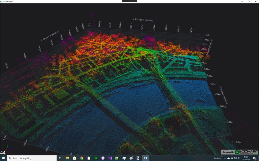
OK so this looks cool but notice in the image below, while the roads and river Thames is clearly visible, the buildings look kind of ghostly and are hard to make out. There’s a lot of data here which is easy to ignore as the point-cloud doesn’t have any solidity to it.
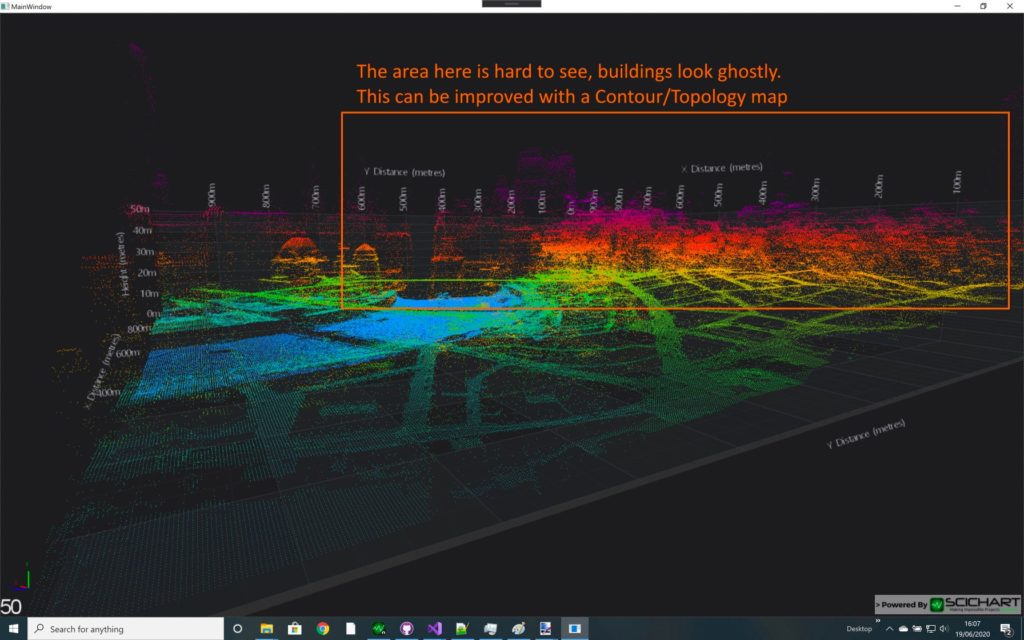
A solution to this is to add contours and topology visualisation to the same 3D graph. SciChart also supports a Surface Mesh 3D Chart type which allows you to visualize a uniform grid of height-values as a surface or mesh, add contours, wireframe and more. We can even add a height-map legend to make it easier for the human-eye to map colour to height.
Transforming the AscData struct earlier into a dataformat to be read by SciChart’s Surface Mesh / Topology map. Here’s the code:
XAML
SciChart WPF requires a SurfaceMeshRenderableSeries3D to render the data as a topology / height-map. I’ve set this to render solid-mesh with contours, and the contours are automatically calculated by our GPU shaders by applying a MeshColorPalette.
<Grid>
<Grid.Resources>
<!-- Define the Surface Mesh colour map. 0 to 1 is mapped to SurfaceMesh.Minimum/Maximum -->
<!-- In this ase DodgerBlue maps to 0m or below and purple to 50m or above -->
<LinearGradientBrush x:Key="ColorMap" StartPoint="0,0" EndPoint="0,1">
<GradientStop Offset="0" Color="DodgerBlue"/>
<GradientStop Offset="0.2" Color="LimeGreen"/>
<GradientStop Offset="0.5" Color="Orange"/>
<GradientStop Offset="0.7" Color="OrangeRed"/>
<GradientStop Offset="1.0" Color="Purple"/>
</LinearGradientBrush>
</Grid.Resources>

<s3D:SciChart3DSurface x:Name="SciChart3DSurface" WorldDimensions="1000,200,1000">

<s3D:SciChart3DSurface.RenderableSeries>

<!-- Renders the contours and topography map -->
<!-- Try different DrawMeshAs modes such as Contours, SolidMesh, SolidMeshWireframe etc -->
<s3D:SurfaceMeshRenderableSeries3D x:Name="surfaceMesh" DrawMeshAs="SolidWithContours"
   MeshPaletteMode="HeightMapInterpolated"
   ContourStroke="Azure" ContourStrokeThickness="2" Minimum="0" Maximum="50"
   Opacity="1">
<s3D:SurfaceMeshRenderableSeries3D.MeshColorPalette>
<s3D:BrushColorPalette Brush="{StaticResource ColorMap}"/>
</s3D:SurfaceMeshRenderableSeries3D.MeshColorPalette>
</s3D:SurfaceMeshRenderableSeries3D>
</s3D:SciChart3DSurface.RenderableSeries>

<!-- X,Y,Z Axis, modifiers omitted for brevity -->

</s3D:SciChart3DSurface>

</Grid>
Code-Behind
In code we simply have to transform the AscData to UniformGridDataSeries3D to display the uniform mesh.
surfaceMesh.DataSeries = await AscReader.ParseToGridDataSeries(lidarData);

// Where ParseToGridDataSeries is implemented as
public static async Task<UniformGridDataSeries3D<float>> ParseToGridDataSeries(AscData lidarData)
{
    UniformGridDataSeries3D<float> uniformGridDataSeries = null;

    await Task.Run(() =>
    {
        // Create the UniformGridDataSeries3D
        uniformGridDataSeries = new UniformGridDataSeries3D<float>(lidarData.NumberColumns, lidarData.NumberRows);
        // Set the step X,Z to AscData.CellSize in metres
        uniformGridDataSeries.StartX = 0;
        uniformGridDataSeries.StepX = lidarData.CellSize;
        uniformGridDataSeries.StartZ = 0;
        uniformGridDataSeries.StepZ = lidarData.CellSize;

        // Fill the 2-dimensional array with height values
        int index = 0;
        for (int z = 0; z < lidarData.NumberRows; z++)
        {
            for (int x = 0; x < lidarData.NumberColumns; x++)
            {
                uniformGridDataSeries.InternalArray[z][x] = lidarData.YValues[index++];
            }
        }
    });

    return uniformGridDataSeries;
}With an opacity of 1.0 the surface mesh looks like this. Height-mapping to the surface-mesh, the colour map and contours are all computed automatically by SciChart, which places contours at set user-defined intervals and maps height-values to colour and displacement in GPU shader programs.
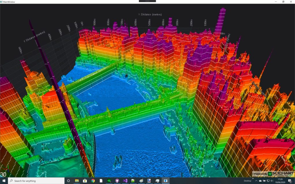
At full opacity it looks nice but it’s hard to see the information about the depth of the field there, so by quickly adding a Legend control with slider for the opacity to the 3D Viewport we can change the transparency of the Point Cloud and Surface Mesh to achieve the desired visual effect. And here it is in all it’s glory below!
You can get the code for this demo from the SciChart.Wpf.Examples Github page.
It turns out the same thing can be achieved on mobile (iOS / Android device). SciChart is a cross-platform data-visualisation library and with its proprietary 3D graphics engine codenamed Visual Xccelerator, it can plot the same kind of data on Windows, iOS, Android, Mac OSX and even browser applications with WebGL.
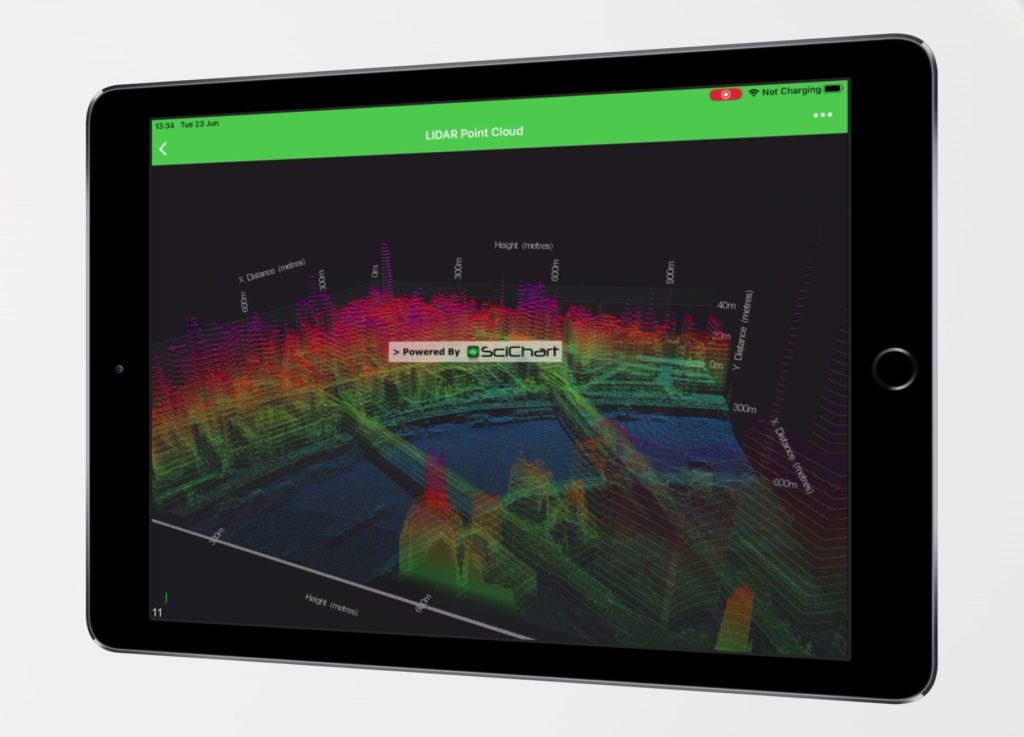
We ported the above LiDAR / GIS Point-cloud and contour topology demo into an iOS app written in Swift in just an hour, and this resulted in the same stunning performance and graphics as our Windows demo. Take a look at the video below to see SciChart.iOS visualising this same dataset.
The source-code for the iOS demo is found at our Github repository under SciChart.iOS.Examples -> Featured Applications -> LiDAR Demo. Download the code today and check it our if you’re interested in this kind of visualisation on iOS.
We mentioned our graphics engine was cross-platform, well, recently we have compiled it to WebAssembly with WebGL to create cutting-edge high performance charts for Javascript and Typescript applications. You can see a preview of SciChart.js – High Performance Javascript Charts.
SciChart.js supports the same types as our Windows and Mobile 2D/3D datavisualisation SDKs. The point-cloud and SurfaceMesh types exist here and we have 3D Charts for Javascript/WebGL applications too.

Using our proprietary cross-platform graphics engine Visual Xccelerator, SciChart.js is able to bring you fast 2D/3D Charts and Data Visualization in the browser with stunning performance through the use of WebGL and WebAssembly.
The source-code looks remarkably similar to our WPF (Windows) and mobile versions, where we load the dataset, create a SciChart3DSurface and use the ScatterRenderableSeries3D with PixelPointMarker to render the dataset. Add a camera and some interactivity modifiers and you have a ready-made Javascript LiDAR visualisation application in just 100 lines of code!
import { createSciChart3DSurface } from "../../../../../../src";
import { CameraController } from "../../../../../../src/Charting3D/CameraController";
import { MouseWheelZoomModifier3D } from "../../../../../../src/Charting3D/ChartModifiers/MouseWheelZoomModifier3D";
import { OrbitModifier3D } from "../../../../../../src/Charting3D/ChartModifiers/OrbitModifier3D";
import { XyzDataSeries3D } from "../../../../../../src/Charting3D/Model/DataSeries/XyzDataSeries3D";
import { Vector3 } from "../../../../../../src/Charting3D/Vector3";
import { NumericAxis3D } from "../../../../../../src/Charting3D/Visuals/Axis/NumericAxis3D";
import { PixelPointMarker3D } from "../../../../../../src/Charting3D/Visuals/PointMarkers/DefaultPointMarkers";
import { ScatterRenderableSeries3D } from "../../../../../../src/Charting3D/Visuals/RenderableSeries/ScatterRenderableSeries3D";
import { TSciChart3D } from "../../../../../../src/types/TSciChart3D";

import { EColor } from "../../../../../../src/types/Color";
import { EColorMapMode, TLinearColorMap } from "../../../../../../src/types/TLinearColorMap";
import { linearColorMapLerp } from "../../../../../../src/utils/colorUtil";
import { AscData, AscReader } from "./AscReader";

export const divElementId = "chart1";

type TMetadata = {
    vertexColorAbgr: number;
    pointScale: number;
};

export const drawExample = async () => {
    const { sciChart3DSurface, wasmContext } = await createSciChart3DSurface(divElementId, 1080, 720);
    sciChart3DSurface.camera = new CameraController(wasmContext, {
        position: new Vector3(300, 300, 300),
        target: new Vector3(0, 50, 0)
    });

    sciChart3DSurface.chartModifiers.add(new MouseWheelZoomModifier3D());
    sciChart3DSurface.chartModifiers.add(new OrbitModifier3D());

    sciChart3DSurface.xAxis = new NumericAxis3D(wasmContext, { axisTitle: "X Axis" });
    sciChart3DSurface.yAxis = new NumericAxis3D(wasmContext, { axisTitle: "Y Axis" });
    sciChart3DSurface.zAxis = new NumericAxis3D(wasmContext, { axisTitle: "Z Axis" });

    const defaultPointMarker = new PixelPointMarker3D(wasmContext, { fill: "#00FF00" });
    // const defaultPointMarker = new SpherePointMarker3D(wasmContext, { size: 1, fill: "#00FF00" });
    const series = new ScatterRenderableSeries3D(wasmContext, { pointMarker: defaultPointMarker });

    series.dataSeries = getData(wasmContext);
    sciChart3DSurface.renderableSeries.add(series);

    return { sciChart3DSurface, wasmContext };
};

function getData(wasmContext: TSciChart3D) {
    // The LinearColorMap type in SciChart allows you to generate a colour map based on a
    // minimum and maximum value, e.g. min=0, max=50 means the gradient brush below is mapped into that range
    //
    const colorMap: TLinearColorMap = {
        Minimum: 0,
        Maximum: 50,
        Mode: EColorMapMode.Interpolated,
        GradientStops: [
            { color: EColor.DodgerBlue, offset: 0 },
            { color: EColor.LimeGreen, offset: 0.2 },
            { color: EColor.Orange, offset: 0.5 },
            { color: EColor.OrangeRed, offset: 0.7 },
            { color: EColor.Purple, offset: 1 }
        ]
    };

    // Read the ASC Lidar data file with optional color map data
    const reader: AscReader = new AscReader(height => colorMapFunction(height, colorMap));
    const ascData: AscData = reader.readFileToAscData("Point cloud");

    // Prepare metadata
    const meta: TMetadata[] = ascData.ColorValues.map(c => ({
        vertexColorAbgr: c,
        pointScale: 0
    }));

    const xyzDataSeries = new XyzDataSeries3D(wasmContext);
    xyzDataSeries.appendRange(ascData.XValues, ascData.YValues, ascData.ZValues, meta);

    return xyzDataSeries;
}

function colorMapFunction(heightValue: number, colorMap: TLinearColorMap): number {
    // Linearly interpolate each heightValue into a colour and return to the ASCReader
    // This will be injected into the SciChart XyzDataSeries3D to colour points in the point-cloud
    return linearColorMapLerp(colorMap, heightValue);
}
SciChart provides high performance real–time chart components on the WPF (Windows), iOS, Android, Xamarin, Mac OSX and Javascript platforms. It is our goal to create the best cross-platform Native WPF, iOS, Android and JavaScript 2D & 3D Charts and Data Visualisation toolkit in the world, focusing on performance, developer productivity, ease of use, depth of features and enterprise-grade tech support.
If you have a question about what SciChart’s WPF, Mobile, or WebGL / WebAssembly Charts can offer you, or if you would like to get a quote, please contact us. Our friendly, helpful support team will be glad to help!
Recent Blogs
![]()
Queens Award for Innovation
Proud winners of the Queens Award for Innovation, 2019. Awarded on account of our innovative graphics engine which underpins the SciChart library and enables our world-beating charting performance
![]()
National Business Awards
Highly Commended for Lloyds National Business Awards, 2019. Awarded on account of our innovative graphics engine and impressive customer base
![]()
National Technology Awards
Awarded “Healthcare Tech of the Year” at the 2025 National Technology Awards – a top UK recognition for breakthrough innovation in technology.

Reviews
SciChart has received hundreds of verified, 3rd party reviews